
EPA’s Water Quality Portal holds more than 430 million records from over 1,000 contributing programs. And cities still get blindsided by contamination events. The gap isn’t data volume. It’s choosing the wrong method for the decision at hand.
If you’re evaluating methods of monitoring water quality for a utility, a discharge permit, an aquaculture site, or a conservation project, the question that matters isn’t “which sensor is best?” It’s: which evidence chain will still hold up when the instrument fouls, conditions shift, or a regulator challenges the result?
After 15 years deploying IoT sensors in industries where “we didn’t know” is an expensive sentence—from air quality monitoring systems to water networks—I can tell you water quality monitoring runs on the same operational truth: speed without accuracy is noise. Accuracy without speed misses the event. The answer is almost never one technology. It’s a layered stack, each method doing what it does best.
Six Families of Water Quality Monitoring
EPA defines water quality monitoring as spanning chemical conditions, physical conditions (temperature, flow, sediment), and biological condition including aquatic communities and test-organism survival. A single program may combine fixed stations, continuous instruments, seasonal campaigns, random sites, and emergency sampling after a spill. No single family covers all of that.
Here’s how the six families compare when you lay them side by side:
| Method Family | What It Measures Well | Main Advantage | Where It Fails |
|---|---|---|---|
| Laboratory sampling (grab/composite) | Nutrients, metals, organics, microbes, PFAS | Broadest analyte coverage, regulatory defensibility | Slow turnaround, costly per sample, misses short events |
| Online sensors and continuous monitoring | Temperature, DO, pH, conductivity, turbidity, algae | Real-time operational feedback, event detection | Drift, fouling, false alarms, calibration burden |
| Remote sensing (satellite/aerial) | Chlorophyll-a, suspended solids, bloom extent, water color | Large-area screening at low marginal cost | Can’t detect toxins directly; affected by clouds and depth |
| Biological assessment | Ecological condition through organism communities | Integrates exposure and habitat effects over time | Slow attribution, seasonal variation, taxonomic expertise |
| eDNA | Genetic traces indicating species, invasives, ecosystem change | Sensitive early signal without capturing organisms | Signal persistence, contamination risk, lab interpretation |
| Citizen and participatory monitoring | Visual condition, field chemistry, biological observations | Dense local coverage, public trust, lower cost | Training consistency, formal regulatory acceptance |
The most common mistake is treating this as a menu where you pick one. It’s a hierarchy. Fast, broad, inexpensive signals (sensors, satellites, trained volunteers) flag attention. Standardized samples and laboratory methods confirm the finding that matters legally or medically. Skip a layer, and you either drown in false alarms or miss the contamination event entirely.
Core Parameters: What to Measure First
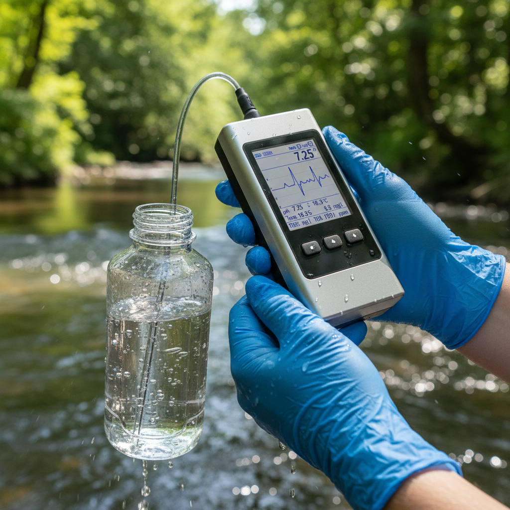
Every monitoring program starts with the same practical question: what are we actually looking for? The answer depends on the water body and the hazard profile, but core field parameters typically include temperature, dissolved oxygen, pH, conductivity, salinity, and turbidity. These reveal the immediate physical and chemical state of the water and can be measured continuously with multiparameter sondes.
From there, programs expand based on risk:
- For drinking water, add microbial indicators, disinfectant residual, lead, copper, and increasingly PFAS. The 2024 PFAS National Primary Drinking Water Regulation sets specific monitoring frequencies and compliance dates running through 2029.
- For industrial discharge, add permit-specific analytes: BOD, TSS, metals, oils. EPA Part 136 methods define the required analytical framework under the Clean Water Act.
- For agricultural runoff, focus on nutrients (nitrogen, phosphorus), sediment, and pesticides. Edge-of-field monitoring with flow-measuring devices captures event-driven loading that periodic sampling misses.
- For aquaculture, ammonia, dissolved oxygen, pH, CO₂, and temperature at high frequency. Minutes matter, not days. A lab result arriving 72 hours later confirms what the farmer already lost.
- For ecological assessment, layer in biological indices, macroinvertebrate communities, and eDNA where species presence and environmental change are the questions.
The principle: start with what tells you the water is immediately dangerous or operationally abnormal. Layer specificity based on the regulatory or ecological question you need to answer. Not every body of water needs a PFAS panel. Every body of water needs someone asking the right first question.
Matching Method to Decision (Not to Budget)
The costliest monitoring failures aren’t caused by cheap equipment. They’re caused by answering the wrong question with the right instrument.
Consider drinking water compliance. Laboratory sampling using approved Part 136 methods remains the backbone for regulated analytes. Online sensors add early warning for treatment optimization and distribution anomalies. EPA’s online water quality monitoring guidance covers source-water stations, distribution-system monitoring, time-series characterization, and event detection. But when PFAS enforcement deadlines arrive in 2027 and 2029, the evidence layer is the certified laboratory result, not the sensor dashboard. The sensor tells you when to sample. The lab tells you what you found.
Harmful algal bloom detection is a different architecture. NASA’s STREAM tool can produce 20-to-30 meter water quality maps and detect anomalies in under six hours by combining Landsat and Sentinel-2 imagery with machine learning. That’s where the bloom is. But EPA is explicit: satellites cannot detect toxin concentrations directly. Toledo’s 2014 microcystin advisory came from a laboratory test, not a satellite image. So the system is: satellite screens, field samples confirm, and public health decides. Three methods, one decision.
Discharge permit compliance is more rigid. NPDES permits specify the sampling method, frequency, and reporting format. A continuous analyzer can improve process control and flag excursions between sampling events, but the permit compliance record requires the method the permit names.
Ecological baseline work calls for biological assessment using macroinvertebrate communities, which integrate exposure over time. eDNA research is expanding rapidly, with recent reviews documenting its use for detecting aquatic organisms and environmental change from genetic traces in water. Neither replaces chemical analysis. Both reveal what chemistry alone misses: the cumulative biological response to everything the water carries.
The pattern across every use case: each decision has a different failure mode and a different time sensitivity. Design the monitoring stack around the decision. Not the other way around.
What Breaks in the Field
This is the section most monitoring guides skip. Sensors get deployed. The dashboard looks clean for two weeks. Then reality sets in.
Every probe drifts over time. pH electrodes age. Dissolved oxygen membranes degrade. A 2024 review identified sensor drift as a persistent source of calibration uncertainty in environmental monitoring, not an edge case. Without a calibration schedule tied to environmental conditions (not just calendar intervals), the data degrades silently. You keep seeing numbers. They stop being accurate.
Biofouling is the next reality check. Submerge any sensor in nutrient-rich water and biology colonizes it: algae, biofilms, sediment coating optical windows and membrane surfaces. Anti-fouling designs help. They don’t eliminate the problem. Manual cleaning visits remain part of the operational burden, and in remote locations, travel time multiplies every visit.
False alarms are subtler but equally dangerous. EPA’s event-detection guidance explicitly evaluates both true detections and invalid alerts. A system that flags everything trains operators to ignore it. A system calibrated too conservatively misses real events. Tuning alarm logic is ongoing work, not a one-time setup.
Then there’s interoperability. A sensor that can’t export data into your existing system (WQX, LIMS, SCADA, or even a shared database) creates an information island. EPA retired the STORET Warehouse in 2018 and consolidated around WQX and the Water Quality Portal for exactly this reason: data that can’t be compared, merged, or reported is operationally dead.
The Flint crisis illustrates what happens when the monitoring design doesn’t match the question. EPA’s response required five distinct sampling objectives, citywide measurement locations, chlorine-residual surveys, and sequential 15-to-20-sample collections in individual homes to evaluate plumbing contributions. A single compliance average wouldn’t have revealed the problem. The lesson extends well beyond lead: define what each sample must answer, publish the location, timing, and sampling rationale, and never assume one metric represents an entire system.
Operational takeaway: budget for maintenance, calibration consumables, alarm tuning, and data integration from day one. If the deployment cost consumes the entire budget, the program fails within a year.
The Full Cost of a Monitoring Program
Market estimates put the water quality monitoring systems market at $5.7 billion in 2024, growing to $8.6 billion by 2030 at a 7.2% CAGR. That growth is real, driven by tightening regulation (especially PFAS), aging infrastructure, and the expanding capability of connected sensors.
But a market number tells you nothing about what a monitoring program actually costs to operate. Here’s what most RFPs leave out:
| Cost Category | What It Includes | Why It Surprises Buyers |
|---|---|---|
| Hardware | Sensors, probes, loggers, enclosures, power | Often the smallest line in a 5-year TCO |
| Calibration and consumables | Reference solutions, replacement membranes, cleaning agents | Frequency depends on environment, not spec sheet |
| Telemetry and connectivity | Cellular plans, satellite backhaul, gateway fees | Recurring cost that scales with sensor count |
| Laboratory confirmation | Certified lab analysis for regulated parameters | Sensors don’t eliminate lab costs; they focus them |
| Software and data management | Dashboard licenses, API access, storage, WQX/LIMS integration | Vendor lock-in risk if data export is limited |
| Maintenance labor | Site visits, cleaning, probe swaps, troubleshooting | Remote sites multiply cost by travel time |
| Response and investigation | Staff time to evaluate alerts, confirm events, report | More sensors generate more alerts to triage |
The honest math: continuous monitoring doesn’t replace laboratory costs. It redirects them. Instead of blind periodic sampling, sensor data triggers targeted lab analysis at the right time and place. That combination costs more upfront than grab-and-ship alone, but it catches events that quarterly sampling misses entirely. For a drinking water utility, one missed contamination event costs orders of magnitude more than a year of continuous monitoring operations.
When evaluating any vendor, request a full bill of materials, calibration and replacement schedule, telemetry fees, laboratory confirmation costs, data integration requirements, and a realistic maintenance calendar. If the vendor can only show you hardware pricing, they’re selling boxes, not a monitoring program.
Where Water Monitoring Is Heading
Three forces are converging in 2026, and each one changes how monitoring programs get designed.
Regulation is accelerating. PFAS reporting requirements begin in April 2027. MCL violation compliance begins in April 2029. EPA’s 2026 proposals may adjust which specific PFAS compounds remain regulated, but the trajectory is clear: more analytes, more frequent monitoring, more defensible data chains. Small systems serving 10,000 or fewer people face the same analytical requirements as large utilities, with far fewer resources to meet them.
IoT and AI are converging beyond simple data logging. IoT-enabled sensing platforms now provide extensive coverage, connectivity, and immediate reporting, while machine learning models detect anomalies faster than manual review. The risk is automation bias: more frequent predictions don’t guarantee better decisions. Data drift, local transferability, and the difference between a proxy signal and a confirmed contaminant concentration must stay visible to operators. The algorithm should trigger the question, not answer it alone.
Interoperability is becoming the real differentiator. The program that wins isn’t the one with the most sensors. It’s the one where sensor data, lab results, satellite imagery, biological indices, and citizen observations flow into a common structure with metadata, uncertainty flags, and a clear chain of custody. EPA’s WQX model points the direction. The vendor that supports open data export and independent confirmation protects the buyer from black-box analytics.
Globally, the urgency is clear. WHO and UNICEF report that 2.1 billion people still lacked safely managed drinking water as of 2024, even as global coverage rose from 68% to 74% over the previous decade. Monitoring capacity must scale alongside water infrastructure, not trail behind it.
Frequently Asked Questions
What is the best method for monitoring water quality?
There is no single best method. Laboratory sampling provides the broadest analyte coverage and strongest regulatory defensibility. Online sensors deliver real-time operational feedback. Remote sensing screens large areas efficiently. Biological methods reveal cumulative ecological effects. The most effective programs layer multiple methods, using fast signals to trigger targeted laboratory confirmation.
Which water quality parameters should be measured first?
Start with core field parameters: temperature, dissolved oxygen, pH, conductivity, and turbidity. These reveal immediate physical and chemical conditions and can be measured continuously. Expand to nutrients, metals, microbes, or PFAS based on the specific water body, regulatory requirements, and known hazard sources in the watershed.
How often should water quality be tested?
Frequency depends on variability and consequence. Source water and distribution systems benefit from continuous or daily monitoring. Status and trend assessments work with seasonal or quarterly campaigns. Emergency sampling addresses spills and floods. Low-frequency grab samples risk missing short contamination pulses entirely.
Can IoT sensors replace laboratory water testing?
No. IoT sensors detect rapid operational changes and trigger alerts, but they measure a limited set of parameters. Regulated analytes like PFAS, heavy metals, and microbial indicators still require certified laboratory analysis. What sensors do is focus lab resources where and when they matter most, reducing blind sampling while improving event detection.
How much does a water quality monitoring program cost?
Hardware is often the smallest component of total cost. A complete budget includes calibration consumables, telemetry fees, software licenses, laboratory confirmation, maintenance labor, and response staffing. Always request a 5-year total-cost-of-ownership breakdown before comparing vendor proposals. If a vendor can only quote hardware, the comparison is incomplete.
What did Flint reveal about monitoring design?
Flint showed that a single compliance metric can mask systemic failure. EPA’s response required five distinct sampling objectives, citywide locations, and sequential home collections to diagnose lead contamination from plumbing. The lesson: define what each sample must answer, and make the sampling rationale, location, and timing transparent.
If your environmental monitoring program needs connected, field-proven sensing for water, soil, temperature, or humidity, explore Datanet’s environmental tracking portfolio. Or talk to our team about what a layered monitoring architecture looks like for your operation.








 +1 508 292 2210

One Response